by Charles Dean Pruitt
(with trigonometric prompting by Katya A.)
ABSTRACT:
The
following is a method to produce equations of various complexities
with real coeffecients
whose solutions generate all prime numbers in an interval.
METHOD:
From
theory and by inspection, composite numbers with similar
factors appear on the
number line in a periodic fashion.
Conversely prime numbers appear on the number
line irregularly as "not composites".
Therefore it is possible to find
a periodic function such as a sine curve or cycloid with
a particular periodicity
which will cross the x-axis (on a two-dimensional Cartesian
coordinate system)
at each integer whose factors correspond to that periodicity.
For purposes of
this argument the sine curve is used because it is the most familiar.
For example:
the sine curve (Sin xPi/2) has an amplitude of one and passes through
the points
on the x-axis (0,0), (2,0), (4,0), (6,0) to infinity, i.e. multiples of two.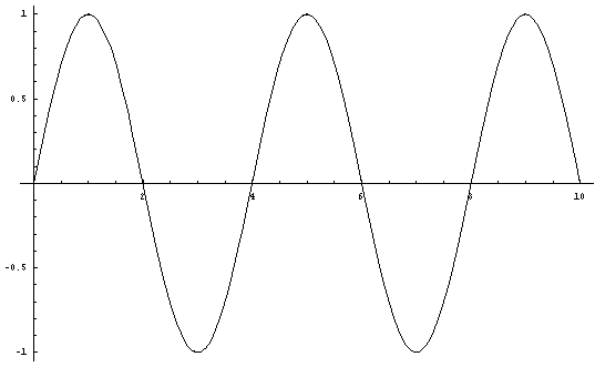
Figure
1.Equation A. y = (Sin xPi/2)
Likewise the sine curve (Sin xPi/3) has an
amplitude of one and passes through
the points on the x-axis (0,0), (3,0), (6,0),
(9,0) to infinity, i.e. multiples of three.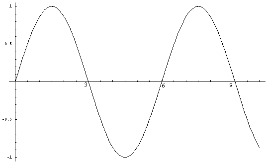
Figure
2. Equation B. y = (Sin xPi/3)
In the same way, the sine curve (Sin xPi/5)
has an amplitude of one and passes through
the points on the x-axis (0,0), (5,0),
(10,0), (15,0) to infinity, i.e. multiples of five.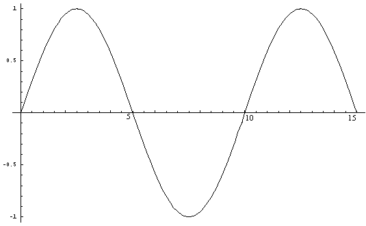
Figure
3. Equation C. y = (Sin xPi/5)
From each of the above three figures it
can be seen that the sine curve passes through
all points on the x-axis which
have its respective prime (and periodicity) as a factor.
When Figure 1 is multiplied
by Figure 2, Figure 4 results.
This is the graph of the curve (Sin xPi/2 * Sin
xPi/3).
It is possible to see that the zero points where the curve crosses the
x-axis
correspond to the integers which have 2 or 3 or both as a factor.
Where
the curve does not intersect the x-axis at the integer values
are integers relatively
prime to two or three.
This is the case up until 'x' equals 25 or five squared.
This
is consistent with standard number theory concerning factorability.
Therefore
for the equation
Sin xPi/2 * Sin xPi/3 = 0,
the points which satisfy the equation
for 'x' are
(2,0), (3,0), (4,0), (6,0), (8,0), (9,0), (10,0), (12,0), (14,0),
(15,0),
(16,0), (18,0), (20,0), (21,0), (22,0), (24,0).
By inspection (see
Figure 4), it can be seen that there is no intersection with
the curve at the
points on the x-axis
(5,0), (7,0), (11,0), (13,0), (17,0), (19,0), (23,0).
This
is confirmed when these values for 'x' are substituted into
the equation and non-zero
answers result.
In effect these are all the primes less than five squared except
two and three.
By the above method is it possible to generate equations which
when solved for
x =0 indicate by elimination that all integers left over are primes.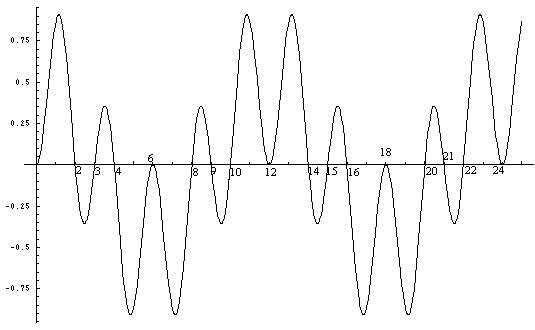
Figure
4. Equation D. y = (Sin xPi/2 * Sin xPi/3)
In order to find the equation
which will provide the curve which
will cross the x-axis for all non-primes less
than seven squared,
it is necessary to multiply (Sin xPi/2 * Sin xPi/3 * Sin xPi/5).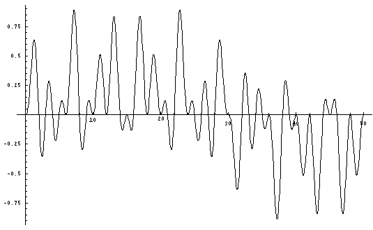
Figure
5. equation E.y = (Sin xPi/2 * Sin xPi/3 * Sin xPi/5)
Although it is not
as clear as on the other graphs,
it is possible to recognize the prime points
on the x-axis.
Therefore when solving for
Sin xPi/2 * Sin xPi/3 * Sin xPi/5
= 0,
the solutions for 'x' (when x<49) comprise all the composite numbers
less
than 49 (7 squared) as well as 2, 3, and 5.
Therefore all the remaining integers
are prime.
With 2, 3, and 5 this constitutes all the primes less than 49.
It
is possible to check this empirically by substitution.
For exceedingly large samples
it is not useful to view a whole graph
because the fine details are not readily
clear.
However it is possible to calculate for a large range
by multiplying
all the consecutive sine curves together.
In the following example the first 27
sine curves (Sin xPi/2) through (Sin xPi/103)
were multiplied together to yield
a graph for the resultant curve
of which 100 units are shown below (figure 6).
That
curve is stated as:
y = [Sin xPi/2 * Sin xPi/3 * Sin xPi/5 * Sin xPi/7 * Sin xPi/11
* Sin xPi/13 * Sin xPi/17 *
Sin xPi/19 * Sin xPi/23 * Sin xPi/29 * Sin xPi/31
* Sin xPi/37 * Sin xPi/41 * Sin xPi/43 *
Sin xPi/47 * Sin xPi/53 * Sin xPi/59
* Sin xPi/61 * Sin xPi/67 * Sin xPi/71 * Sin xPi/73 *
Sin xPi/79 * Sin xPi/83
* Sin xPi/89 *Sin xPi/97 *Sin xPi/101 * Sin xPi/103]
(Equation F.)
Solving
the resultant equation for zero yields all the
composite numbers up to 103 squared
(10609) and
consequently by elimination all of the primes less than 10609.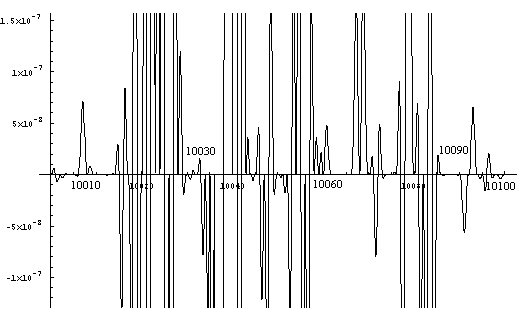
Figure
6. Equation F. y = (Sin xPi/2* Sin xPi/3 * ... * Sin xPi/101 * Sin xPi/103)
For
purposes of illustration a small segment of the graph
is blown up (figure 7) to
shown the fine detail and confirm
visually that indeed the resulting curve crosses
the x-axis
at all the composite numbers and not at any of the primes.
However
for all values of 'x' which satisfy the equation,
results can only be derived
by solving for zero.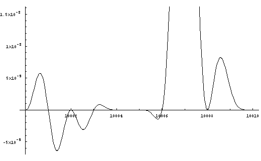
Figure
7. Equation F. Detail 10000 to 10010
It appears from this segment of the
graph that 10007 and 10009
are prime (and constitute a prime pair). This is indeed
the case.
The curve between 10004 and 10006 has an amplitude of less than one
ten-billionth.
With further magnification (see Figure 8) details as fine one part
in a trillion
are resolved and indicate 10005 is composite.
(Of course there
are easier methods to determine
compositeness of numbers ending in 5.)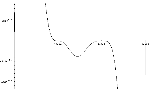
Figure
8. Equation F. Detail 10003-10006
PROOF
Each periodic function as
defined above intersects
the x-axis at points that correspond to all
the integers
divisible by that function when y=0.
Sin xPi/2=0 represents all integers divisible
by 2.
Sin xPi3=0 represents all integers divisible by 3.
Sin xPi/5=0 represents
all integers divisible by 5.
When two functions are multiplied together,
they
will show up all the zeroes because 0 times anything is 0 .
Sin xPi/2 * Sin xPi/3=0
represents all integers divisible by 2 and/or 3.
Sin xPi/3 * Sin xPi/5=0 represents
all integers divisible by 3 and/or 5.
Sin xPi/5 * Sin xPi/7=0 represents all integers
divisible by 5 and/or 7.
There is not duplication because 0 times 0 is 0
and
hence there would be only one point indicated instead of two.
Likewise the same
argument applies when many sine curves are multiplied together.
When all sine
curves (each with periodicity corresponding to a prime and
all such curves up
to and including that whose periodicity is
less than or equal to the square root
of the largest number
in the sample space being tested) are multiplied together,
the
resultant equation gives each composite number one time
when the equation is solved
for zero.
Discarding these from the set of integers leaves the primes.
In practice
this has become a formulaic Sieve of Erastathenes.
This not a true equation whose
solutions yield primes.
To do this it is necessary to choose periodic equations
which
are not as tidy as a Sine curve.
This is done by using a similar curve (in this
case a Cosine curve)
and translating the axes. According to the parameters set
out above,
a necessary condition is that the curve intersects the x-axis in a
periodic fashion
and at the points where it intersects exhibits a desired characteristic.
In
this case relative primality.
Consider the case of relative primality with respect
to two.
This is straightforward since it is possible to construct a curve that
intersects
the x-axis at points relatively prime wih respect to two (i.e. 1, 3,
5, 7, etc.).
Below is a Cosine curve with the axes translated such that the troughs
of the
Cosine curve intersect the x-axis at integers relatively prime to two.
The
equation of this curve is y = 1+Cos(Pi(x))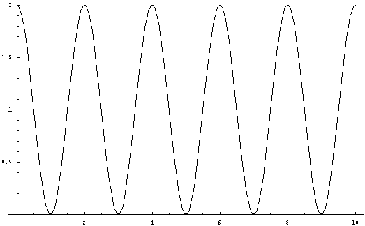
Figure
9. Equation G. y = 1+Cos(Pi(x))
From Figure 9 it is possible to see that
for x = 0, y assumes values relatively prime to 2.
Likewise it is possible to
choose similar Cosine curves for other integers.
However to do this for three
for example, it is necessary to use multiple curves since a
single Cosine curve
will not touch the x-axis at every integer relatively prime to three.
The first
curve is y = 1+Cos(Pi(2x+5)/3)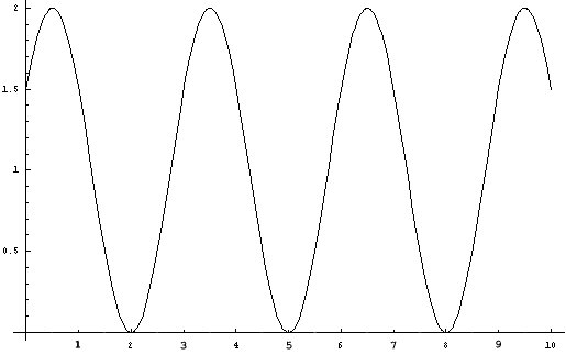
Figure
10. Equation H. y = 1+Cos(Pi(2x+5)/3)
Observe that this curve intersects
the x-axis at values 3a + 2
and are all relatively prime to 3.
The second curve
is y = 1+Cos(Pi(2x+7)/3)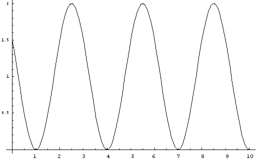
Figure
11. Equation I. y = 1+Cos(Pi(2x+7)/3)
Observe that this curve intersects
the x-axis at values 3a + 1
and are all relatively prime to 3.
When y = 1+Cos(Pi(2x+5)/3)
and y = 1+Cos(Pi(2x+7)/3)
are multiplied together the equation is
y = 1 + Cos(Pi2x+5)/3)
+ Cos(Pi(2x+7)/3) + Cos(Pi(2x+5)/3)*Cos(Pi(2x+7)/3).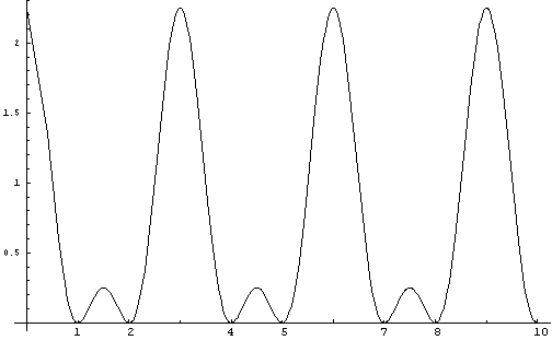
Figure
12. Equation J.
y = 1 + Cos(Pi(2x+5)/3) + Cos(Pi(2x+7)/3) + Cos(Pi(2x+5)/3)*Cos(Pi(2x+7)/3)
Observe
that this curve intersects the x-axis at values 3a + 1 and 3a + 2
and are all
relatively prime to 3.
To get an equation which when solved for y = 0 yields values
of "x" which are
relatively prime to two and three it is necessary to
add Equation G and Equation J.
If y = 1 + Cos(Pi(2x+5)/3) + Cos(Pi(2x+7)/3) +
Cos(Pi(2x+5)/3)*Cos(Pi(2x+7)/3)
is added to y = 1+Cos(Pi(x) the resulting equation
is
y = 2+ Cos(Pi(2x+5)/3) + Cos(Pi(2x+7)/3) + Cos(Pi(x)) + Cos(Pi(2x+5)/3)*Cos(Pi(2x+7)/3).
When
solved for y = 0, this equation gives values relatively prime to infinity and
gives
prime values for "x" when y = 0 when x<5².
As is readily apparent,
this equation is unwieldy and
not amenable for searching for primes.
The graph
of this equation is: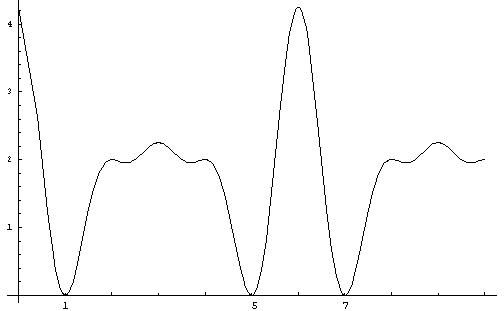
Figure
13. Equation K.
y = 2+ Cos(Pi(2x+5)/3) + Cos(Pi(2x+7)/3) + Cos(Pi(x)) + Cos(Pi(2x+5)/3)*Cos(Pi(2x+7)/3)
The
corresponding equations which describe a curve on which the zero points with
respect
to "y" are relatively prime to five are derived from the following equations:
y
= 1+Cos(Pi(2x+7)/5)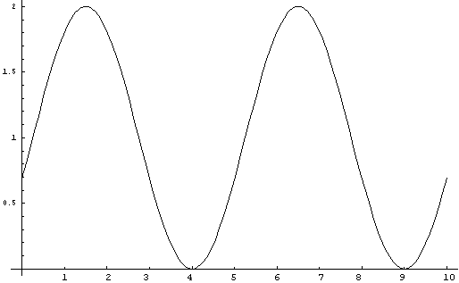
Figure
14. Equation L. y = 1+Cos(Pi(2x+7)/5)
y = 1+Cos(Pi(2x+9)/5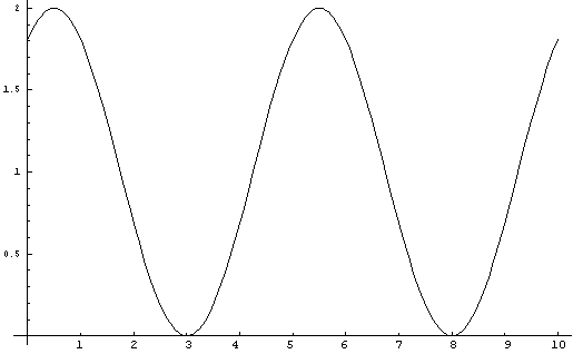
Figure
15. Equation M. y = 1+Cos(Pi(2x+9)/5)
y = 1+Cos(Pi(2x+11)/5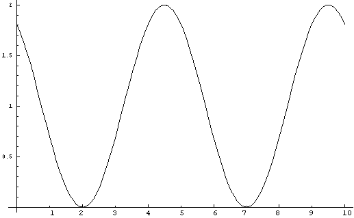
Figure
16. Equation N. y = 1+Cos(Pi(2x+11)/5)
y = 1+Cos(Pi(2x+13)/5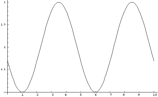
Figure
17. Equation O. y = 1+Cos(Pi(2x+13)/5)
When the four equations are multiplied
together the resulting equation is:
y = 1 + Cos[Pi(7 + 2x)/5] + Cos[Pi(9 +
2x)/5] + Cos[Pi(7 + 2x/5] * Cos[Pi(9 + 2x)/5] +
Cos[Pi(11 + 2x)/5] + Cos[Pi(7
+ 2x)/5] * Cos[Pi(11 + 2x)/5] +
Cos[Pi(9 + 2x)/5] * Cos[Pi(11 + 2x)/5] +
Cos[Pi(7
+ 2x)/5] * Cos[Pi(9 + 2x)/5] * Cos[Pi(11 + 2x)/5] +
Cos[Pi(13 + 2x)/5] + Cos[Pi(7
+ 2x)/5] * Cos[Pi(13 + 2x)/5] +
Cos[Pi(9 + 2x)/5] * Cos[Pi(13 + 2x)/5] +
Cos[Pi(7
+ 2x)/5] * Cos[Pi(9 + 2x)/5] * Cos[Pi(13 + 2x)/5] +
Cos[Pi(11 + 2x)/5] * Cos[Pi(13
+ 2x)/5] +
Cos[Pi(7 + 2x)/5] * Cos[Pi(11 + 2x)/5] * Cos[Pi(13 + 2x)/5] +
Cos[Pi(9
+ 2x)/5] * Cos[Pi(11 + 2x)/5] * Cos[Pi(13 + 2x)/5)] +
Cos[Pi(7 + 2x)/5] * Cos[Pi(9
+ 2x)/5] * Cos[Pi(11 + 2x)/5] * Cos[Pi(13 + 2x)/5]
The graph for this is: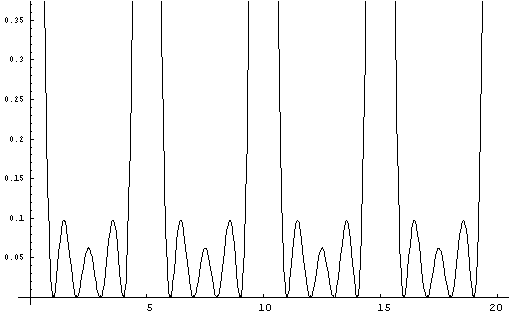
Figure
18. Equation P.
y = 1 + Cos[Pi(7 + 2x)/5] + Cos[Pi(9 + 2x)/5] + Cos[Pi(7 + 2x/5]
* Cos[Pi(9 + 2x)/5] +
Cos[Pi(11 + 2x)/5] + Cos[Pi(7 + 2x)/5] * Cos[Pi(11 + 2x)/5]
+
Cos[Pi(9 + 2x)/5] * Cos[Pi(11 + 2x)/5] +
Cos[Pi(7 + 2x)/5] * Cos[Pi(9 +
2x)/5] * Cos[Pi(11 + 2x)/5] +
Cos[Pi(13 + 2x)/5] + Cos[Pi(7 + 2x)/5] * Cos[Pi(13
+ 2x)/5] +
Cos[Pi(9 + 2x)/5] * Cos[Pi(13 + 2x)/5] +
Cos[Pi(7 + 2x)/5] * Cos[Pi(9
+ 2x)/5] * Cos[Pi(13 + 2x)/5] +
Cos[Pi(11 + 2x)/5] * Cos[Pi(13 + 2x)/5] +
Cos[Pi(7
+ 2x)/5] * Cos[Pi(11 + 2x)/5] * Cos[Pi(13 + 2x)/5] +
Cos[Pi(9 + 2x)/5] * Cos[Pi(11
+ 2x)/5] * Cos[Pi(13 + 2x)/5)] +
Cos[Pi(7 + 2x)/5] * Cos[Pi(9 + 2x)/5] * Cos[Pi(11
+ 2x)/5] * Cos[Pi(13 + 2x)/5]
When Equation P is added to Equation K, the
resulting equation when solved for zero,
yields an infinite number of values
of "x" which are relatively prime with respect to
2, 3 and 5. For values
of "x" less than 7², "x" is prime.
This equation is:
y =
3 + Cos[Pi(2x+5)/3] + Cos[Pi(2x+7)/3] + Cos[Pi(x)] + Cos[Pi(2x+5)/3]*Cos[Pi(2x+7)/3]
+
Cos[Pi(7 + 2x)/5] + Cos[Pi(9 + 2x)/5] + Cos[Pi(7 + 2x/5] * Cos[Pi(9 + 2x)/5] +
Cos[Pi(11
+ 2x)/5] + Cos[Pi(7 + 2x)/5] * Cos[Pi(11 + 2x)/5] +
Cos[Pi(9 + 2x)/5] * Cos[Pi(11
+ 2x)/5] +
Cos[Pi(7 + 2x)/5] * Cos[Pi(9 + 2x)/5] * Cos[Pi(11 + 2x)/5] +
Cos[Pi(13
+ 2x)/5] + Cos[Pi(7 + 2x)/5] * Cos[Pi(13 + 2x)/5] +
Cos[Pi(9 + 2x)/5] * Cos[Pi(13
+ 2x)/5] +
Cos[Pi(7 + 2x)/5] * Cos[Pi(9 + 2x)/5] * Cos[Pi(13 + 2x)/5] +
Cos[Pi(11
+ 2x)/5] * Cos[Pi(13 + 2x)/5] +
Cos[Pi(7 + 2x)/5] * Cos[Pi(11 + 2x)/5] * Cos[Pi(13
+ 2x)/5] +
Cos[Pi(9 + 2x)/5] * Cos[Pi(11 + 2x)/5] * Cos[Pi(13 + 2x)/5)] +
Cos[Pi(7
+ 2x)/5] * Cos[Pi(9 + 2x)/5] * Cos[Pi(11 + 2x)/5] * Cos[Pi(13 + 2x)/5]
The graph
for this is: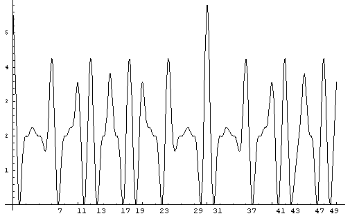
Figure
19. Equation Q.
y = 3 + Cos[Pi(2x+5)/3] + Cos[Pi(2x+7)/3] + Cos[Pi(x)] + Cos[Pi(2x+5)/3]*Cos[Pi(2x+7)/3]
+
Cos[Pi(7 + 2x)/5] + Cos[Pi(9 + 2x)/5] + Cos[Pi(7 + 2x/5] * Cos[Pi(9 + 2x)/5] +
Cos[Pi(11
+ 2x)/5] + Cos[Pi(7 + 2x)/5] * Cos[Pi(11 + 2x)/5] +
Cos[Pi(9 + 2x)/5] * Cos[Pi(11
+ 2x)/5] +
Cos[Pi(7 + 2x)/5] * Cos[Pi(9 + 2x)/5] * Cos[Pi(11 + 2x)/5] +
Cos[Pi(13
+ 2x)/5] + Cos[Pi(7 + 2x)/5] * Cos[Pi(13 + 2x)/5] +
Cos[Pi(9 + 2x)/5] * Cos[Pi(13
+ 2x)/5] +
Cos[Pi(7 + 2x)/5] * Cos[Pi(9 + 2x)/5] * Cos[Pi(13 + 2x)/5] +
Cos[Pi(11
+ 2x)/5] * Cos[Pi(13 + 2x)/5] +
Cos[Pi(7 + 2x)/5] * Cos[Pi(11 + 2x)/5] * Cos[Pi(13
+ 2x)/5] +
Cos[Pi(9 + 2x)/5] * Cos[Pi(11 + 2x)/5] * Cos[Pi(13 + 2x)/5)] +
Cos[Pi(7
+ 2x)/5] * Cos[Pi(9 + 2x)/5] * Cos[Pi(11 + 2x)/5] * Cos[Pi(13 + 2x)/5]
When
Equation Q is plotted from zero to ninety,
it is obvious that it has a period
of thirty (2 x 3 x 5).
Similarly the next curve would have a periodicity of 210
(2 x 3 x 5 x7).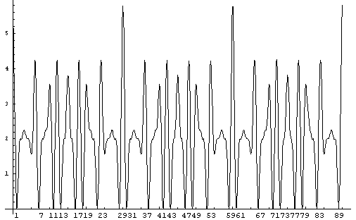
Figure
20. Equation Q plotted to 90.
COMMENTARY
Are these true
formulae for generating primes?
Yes.
Solve for zero and they generate integer
values of all the numbers
that are prime less than a certain value.
For
example: if the graphs are summed for the family of curves
up to and including
1 + Cos[Pi(A + 2x)/P(n)] then
all primes less than P(n+1) are the solutions of
the equation.
Are they useful formulae?
They are computationally intensive,
but the idea of multiplying
periodic equations together and solving for zero has
utility value.
Suppose periodic equations could be constructed that were inherently
simple
and when multiplied together were likewise simple.
The restraint of
computational intensity would be diminished
with a clever enough set of periodic
equations.
If non-trigonometric periodic equations could be found,
it might
produce a polynomial which could be solved for
and produce integer roots all of
which are composite.
From this would come all the primes via solution of a polynomial
and
subsequent cataloging those integers which don't solve the equation.
Of other
utility value is the possibility to demonstrate via
substitution
in these equations a number's primality or compositeness.
Again there is the
computational intensiveness.
By way of example, Equation F can test
all numbers
less than